68 Machine Learning: Introduction

68.1 What is Machine Learning?

Over the next three weeks, we’ll explore various concepts and techniques relating to machine learning. Some of this will be new to you, but there will also be many familiar ideas (such as regression and cluster analysis) that we have covered earlier in B1705 and B1700.

Hopefully, you will see that ML is (in part) a very similar process to the kind of model-building we’ve already encountered.

Definition and Scope

Machine learning (ML) is a subset of artificial intelligence (AI) that focuses on building systems that learn from data.

Instead of being explicitly programmed to perform a task, these systems improve their performance on a task over time with experience.

In essence, the predictive model is created and is then tested in real-time. Based on its performance in real-time, it is continually updated to maintain and improve its performance. It continues to ‘learn’ over time.

In 2024, ML is at the heart of many cutting-edge technologies and is pivotal in sectors such as finance, healthcare, and e-commerce, where it underpins recommendations, decision-making processes, and predictive analytics.

Types of machine learning

There are three main forms of ML:

Supervised Learning

Supervised learning is a category of machine learning where the algorithm learns from labeled training data, using it to predict outcomes or classify data into different categories.

We first encountered this approach when we learned about Discriminant Analysis earlier in the module.

This method involves a teacher-supervisor who presents the machine with input-output pairs, where the machine must learn to map inputs to outputs.
The goal is to generalise from the training data to new, unseen situations.
Common applications of supervised learning include spam detection in email, weather forecasting, and facial recognition.
Supervised learning models include algorithms like linear regression for continuous output or logistic regression, decision trees, and neural networks for categorical output.

For example, in linear regression, we ‘train’ a model to learn the impact that one or more IVs have on a DV. The model ‘learns’ whether their effect is significant, and to what extent changes in one IV impact the DV.

in this example, the regression model identifies that both IVs are significant (p < 0.05) and provides an estimate of their impact (-3.2 and -1.5). This can then be used to construct an equation that allows future performance to be predicted.

Code

# Supervised learning example with linear regression
library(caret)
library(tidyverse)

data("mtcars")
model <- lm(mpg ~ wt + cyl, data = mtcars)
summary(model)


Call:
lm(formula = mpg ~ wt + cyl, data = mtcars)

Residuals:
    Min      1Q  Median      3Q     Max 
-4.2893 -1.5512 -0.4684  1.5743  6.1004 

Coefficients:
            Estimate Std. Error t value Pr(>|t|)    
(Intercept)  39.6863     1.7150  23.141  < 2e-16 ***
wt           -3.1910     0.7569  -4.216 0.000222 ***
cyl          -1.5078     0.4147  -3.636 0.001064 ** 
---
Signif. codes:  0 '***' 0.001 '**' 0.01 '*' 0.05 '.' 0.1 ' ' 1

Residual standard error: 2.568 on 29 degrees of freedom
Multiple R-squared:  0.8302,    Adjusted R-squared:  0.8185 
F-statistic: 70.91 on 2 and 29 DF,  p-value: 6.809e-12

Unsupervised Learning

In this type of model, the system tries to learn the structure or distribution of data without labels. It’s more about finding patterns and relationships in data.

Remember: in supervised learning we told the model what our inputs (IVs) and output (DV) were. That kind of definition doesn’t exist in unsupervised learning - the algorithm is left to find patterns and associations by itself.

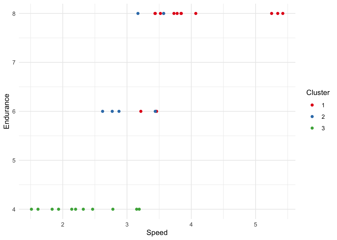
Clustering (which we covered in week two) is a common example where we ask the algorithm to find associations between variables, rather than define them. In this case, we ask the algorithm to find out the best way to ‘group’ different types of car: we don’t tell it what group each car belongs to.

Code

# Unsupervised learning example with clustering
library(cluster)
data <- scale(mtcars)  # Normalizing data
fit <- kmeans(data, 3)  # K-means clustering with 3 clusters
#print(fit$cluster)

mtcars$cluster <-fit$cluster

mtcars$cluster <- as.factor(mtcars$cluster)

# Create a scatter plot using ggplot
ggplot(mtcars, aes(x = wt, y = cyl, color = factor(cluster))) +
  geom_point() +  # Add points
  labs(color = "Cluster", x = "Speed", y = "Endurance") + # Labeling
  theme_minimal() +  # Minimal theme
  scale_color_brewer(palette = "Set1")  # Use a color palette for better distinction

Reinforcement Learning

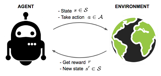
Reinforcement learning (RL) is a more complex type of unsupervised machine learning where an ‘agent’ learns to make decisions by performing actions in an environment to achieve a goal.

The agent receives feedback through rewards or penalties, guiding it to ‘learn’ the best strategy, known as a policy, to maximise cumulative rewards over time.

Unlike supervised learning, where the model learns from a dataset containing the correct answers, RL involves learning optimal actions through trial and error and interaction with the environment. This method is particularly powerful in scenarios where the right sequence of actions is critical for success, such as in game playing, robotics, and navigation tasks, where the agent must make a series of decisions that build upon each other to achieve a long-term objective.